Your Brain Has a Direction. Granger Causality Finds It.

Correlation Has a Dirty Secret: It Can't Tell You Who Started Talking
Here's something that might bother you once you notice it.
Most of what we know about how brain regions work together comes from measuring correlation. Two regions go up and down at the same time, so we say they're "connected." This is the foundation of functional connectivity analysis, and it has produced genuinely important science over the past few decades.
But correlation has a problem. A big one.
If I tell you that the activity at your left frontal cortex and your right parietal cortex are strongly correlated during a working memory task, you know something interesting is happening. Those two regions are doing something in sync. But you don't know the most important thing: which region is talking and which region is listening.
Is the frontal cortex sending instructions to the parietal cortex? Is the parietal cortex feeding information forward to the frontal cortex? Are they both receiving orders from some third region entirely? Correlation can't tell you. It's blind to direction.
This is like knowing that two people are having a conversation but having no idea who brought up the topic. In neuroscience, the direction of information flow between brain regions isn't a minor detail. It's often the whole story. A frontal region driving a sensory region means top-down attention. A sensory region driving a frontal region means bottom-up perception. Same two regions, same synchronization, completely different cognitive processes.
So how do you figure out the direction? That's where a Nobel Prize-winning economist accidentally gave neuroscience one of its most powerful tools.
An Economist Walks Into a Brain Lab
In 1969, a British economist named Clive Granger published a paper that had nothing to do with the brain. He was trying to solve a practical problem in economics: if you have two time series, like the price of wheat and the price of bread, how do you determine whether one actually influences the other, or whether they just happen to move together?
His solution was elegant, almost deceptively simple. Here's the core idea.
Say you want to know if time series X causes time series Y. First, build the best prediction model you can for Y using only Y's own past values. Basically, use yesterday's Y, the day before's Y, and so on, to predict today's Y. Measure how well that model performs.
Now build a second model. This time, predict Y using both Y's own past AND X's past values. If the second model is significantly better, if knowing what X was doing in the past genuinely improves your ability to predict what Y does next, then X "Granger-causes" Y.
That's it. That's the whole concept.
Granger wasn't claiming that X truly causes Y in the deep philosophical sense. He was carefully precise about this. He was saying that X contains information about Y's future that Y itself doesn't contain. The past of X carries predictive power for Y above and beyond what Y's own past provides.
This distinction between "true" causation and "predictive causation" is important, and we'll come back to it. But first, let's talk about why neuroscientists got very excited about this idea.
Why Your Brain Is the Perfect Place for Granger Causality
EEG data is, at its heart, a collection of time series. Each electrode on your scalp records voltage fluctuations over time, sampled hundreds of times per second. If you have 8 electrodes, you have 8 simultaneous time series, each one capturing the aggregate electrical activity of the brain tissue beneath it.
And those time series are not independent. Brain regions communicate constantly, passing information back and forth through white matter tracts, thalamocortical loops, and cortico-cortical connections. The signals at different electrodes rise and fall in patterns that reflect this underlying communication.
This is exactly the setup Granger causality was designed for. Two (or more) time series, potentially influencing each other, unfolding in time. The question is which one leads and which one follows.
When researchers first applied Granger causality to EEG data in the early 2000s, the results were striking. You could actually see directed information flow between brain regions during cognitive tasks. Visual cortex driving frontal cortex during perception. Frontal cortex driving sensory cortex during attention. The direction of influence changing dynamically as the brain switched between processing modes.
This was something fundamentally new. Not just "these regions are active together" but "this region is feeding information to that one."
How Granger Causality Actually Works in EEG (The Math, Made Human)
The standard implementation of Granger causality for EEG uses something called a vector autoregressive (VAR) model. Don't let the name scare you. The concept is straightforward once you break it apart.
An autoregressive model predicts the current value of a signal based on its own past values. "Auto" means self. "Regressive" means using past data to predict future data. So an autoregressive model for EEG channel Y says: "the voltage at Y right now is some weighted combination of what Y was doing at the previous 5, 10, or 20 time points, plus some random noise."
A vector autoregressive model does the same thing, but for multiple channels at once, and each channel can be predicted using the past values of ALL channels. So the voltage at Y right now is predicted by Y's own recent past PLUS X's recent past PLUS Z's recent past, and so on for every channel in the model.
Now you run the comparison. Build a model for channel Y using only Y's own past (the "restricted" model). Build another model using Y's past AND X's past (the "unrestricted" model). Compare the prediction errors. If the unrestricted model produces significantly smaller errors, X Granger-causes Y.
You can run this test for every pair of channels, in both directions. X to Y, and Y to X. This gives you a complete directed connectivity map: a matrix showing how much each brain region's past predicts each other region's future.
- Record multi-channel EEG with electrodes over regions of interest
- Preprocess the data (filter, remove artifacts, ensure stationarity)
- Select the model order (how many past time points to include)
- Fit the restricted model (each channel predicted by only its own past)
- Fit the unrestricted model (each channel predicted by all channels' past)
- Compare prediction errors using an F-test or likelihood ratio test
- Determine significance (often with surrogate data or permutation testing)
- Repeat for all channel pairs to build a directed connectivity matrix
The Model Order Problem: How Far Back Should You Look?
One critical decision in Granger causality analysis is the model order, the number of past time points you include in the model. This matters more than it might seem.
If the model order is too low, you miss information. Maybe the influence from X to Y has a delay of 50 milliseconds, but your model only looks back 10 milliseconds. You'll miss the relationship entirely.
If the model order is too high, you overfit. Your model starts memorizing noise rather than capturing genuine predictive relationships. The statistical test loses power, and you might miss real effects or find spurious ones.
For EEG sampled at 256Hz, researchers commonly use model orders corresponding to 10-50 milliseconds of data, which translates to roughly 3-13 time points. The exact choice often relies on information criteria like the Akaike Information Criterion (AIC) or the Bayesian Information Criterion (BIC), which balance model fit against model complexity.
Think of it like choosing how far back in a conversation to listen when trying to predict what someone will say next. Too few words and you lack context. Too many and you're overloaded with irrelevant history. There's a sweet spot, and these statistical criteria help you find it.
Spectral Granger Causality: Finding Direction at Specific Frequencies
Here's where things get really interesting.
Standard Granger causality gives you one number per channel pair: an overall measure of directed influence. But the brain doesn't communicate on a single channel. Different frequency bands carry different types of information. Alpha oscillations (8-13 Hz) handle sensory gating and attention. Beta oscillations (13-30 Hz) support motor planning and status quo maintenance. Gamma oscillations (30-100+ Hz) bind distributed features into coherent percepts.
So when frontal cortex Granger-causes parietal cortex, you want to know: at what frequency? Is the frontal cortex sending alpha-band signals to suppress irrelevant sensory input? Or is it sending gamma-band signals to bind a visual scene together? These are completely different neural processes, and time-domain Granger causality lumps them all into one number.
Spectral Granger causality solves this by decomposing the directed influence into frequency components. The mathematical foundation comes from decomposing the VAR model into the frequency domain using Fourier transforms, which yields a frequency-resolved version of the Granger causality measure.
The results are illuminating. Studies using spectral Granger causality have revealed that:
- Top-down attention flows from frontal to sensory cortex primarily in the alpha and beta bands
- Bottom-up sensory processing flows from sensory to frontal cortex primarily in the gamma band
- During working memory maintenance, prefrontal cortex drives parietal cortex in the theta band
- Motor preparation involves beta-band directed flow from premotor to primary motor cortex
This frequency-specific directionality has become one of the most important findings in modern cognitive neuroscience. It suggests that the brain uses different frequencies as different communication channels, with information flowing in different directions at different frequencies simultaneously.
Your brain runs a two-way highway between frontal and sensory regions, and different lanes of that highway use different frequencies. When your frontal cortex needs to suppress distracting input, it sends alpha-band signals backward to sensory cortex, essentially shushing it. When your sensory cortex detects something important, it sends gamma-band signals forward to frontal cortex, essentially shouting for attention. Both happen at the same time, between the same regions, in opposite directions, on different frequencies. Granger causality is what revealed this. Without directionality, you'd just see "frontal and sensory cortex are connected." With it, you see a sophisticated two-channel communication protocol that the brain evolved over millions of years.
Granger Causality vs Other Connectivity Methods: Which Is Better?
Granger causality isn't the only tool for studying brain connectivity. It exists in a landscape of methods, each with different strengths. Here's how they compare.
| Method | Type | Directionality | Frequency-Resolved | Best For |
|---|---|---|---|---|
| Coherence | Functional | No | Yes | Measuring synchronization strength between regions |
| Phase-Locking Value | Functional | No | Yes | Detecting consistent phase relationships across trials |
| Granger Causality | Effective | Yes | Yes (spectral version) | Detecting directed information flow in time series |
| Transfer Entropy | Effective | Yes | No (time-domain) | Detecting nonlinear directed dependencies |
| Dynamic Causal Modeling | Effective | Yes | No (model-based) | Testing specific hypotheses about network architecture |
| Partial Directed Coherence | Effective | Yes | Yes | Frequency-resolved directed connectivity in multivariate data |
| Directed Transfer Function | Effective | Yes | Yes | Similar to PDC with different normalization |
The distinction between functional connectivity and effective connectivity is fundamental here. Functional connectivity measures statistical dependencies, like correlation or coherence, without implying a direction of influence. It tells you that two regions are doing something together. Effective connectivity measures directed influence, telling you which region is driving which. Granger causality, transfer entropy, and dynamic causal modeling are all effective connectivity methods.
Two close relatives of Granger causality deserve special mention. Partial directed coherence (PDC) and the directed transfer function (DTF) are both derived from the same VAR model framework as Granger causality but are formulated directly in the frequency domain. PDC emphasizes direct connections between regions (filtering out indirect paths), while DTF captures both direct and indirect influence. Many EEG researchers prefer these methods over standard spectral Granger causality because they handle multivariate data more naturally.
The Limitations You Actually Need to Know About
Granger causality is powerful, but it has real limitations that you can't ignore. Understanding these isn't just academic caution. Getting them wrong will lead you to genuinely incorrect conclusions about how your brain works.
Volume Conduction: The Ghost in the Machine
This is the big one. EEG signals are measured on the scalp, but they originate inside the brain. Electrical fields spread through brain tissue, skull, and scalp before reaching the electrodes. This means a single neural source deep in the brain can project its activity onto multiple scalp electrodes simultaneously.
The problem for Granger causality: if two electrodes are both picking up the same underlying source (with slightly different delays due to different propagation paths), you can see apparent Granger causality between them even though there's no actual directed communication between two brain regions. One source, two electrodes, fake directionality.
Researchers address this in several ways. Some use source localization algorithms to estimate the activity of cortical sources underneath the scalp and then compute Granger causality between the estimated sources rather than the raw scalp signals. Others use the imaginary part of coherence or time-reversed Granger causality as controls. Still others simply acknowledge the limitation and interpret results cautiously.
The Confound of Common Drivers
If a hidden third region drives both X and Y with different delays, X might appear to Granger-cause Y even though X and Y have no direct connection. X just happens to receive its input from the common driver slightly earlier.
In a two-channel analysis, this is nearly impossible to distinguish from genuine directed influence. Multivariate Granger causality (using all available channels simultaneously) helps by conditioning on other observed channels, but it can't account for sources you're not measuring.
Stationarity Assumptions
Standard Granger causality assumes that the statistical properties of the signals don't change over time. Brain signals are famously non-stationary. Your neural dynamics shift from moment to moment as you think, attend, and react.
Researchers handle this by analyzing short windows of data (where stationarity is more plausible) or by using time-varying versions of Granger causality that allow the model parameters to evolve. But short windows mean fewer data points, which reduces statistical power. It's a constant tradeoff.
Linearity
The standard VAR-based Granger causality assumes linear relationships between signals. Real neural interactions include plenty of nonlinear dynamics. Transfer entropy, an information-theoretic cousin of Granger causality, captures nonlinear dependencies but requires more data and is more computationally expensive.
Putting It to Work: What Researchers Have Found
Despite its limitations, Granger causality has produced findings that reshaped our understanding of brain communication. Here are some of the most compelling.
Visual attention routing. Researchers used spectral Granger causality to show that when you pay attention to something in your left visual field, your right frontal cortex increases its gamma-band Granger-causal influence on right visual cortex. Attention isn't just "turning up the volume" in sensory cortex. It's the frontal cortex actively sending signals that modulate sensory processing. This was one of the first demonstrations that attention is a directed, frequency-specific top-down process.
The default mode network at rest. During quiet rest with eyes closed, Granger causality reveals a rich pattern of directed information flow between midline frontal and parietal regions, the core hubs of the default mode network. This flow changes direction during the transition from rest to task engagement, with parietal-to-frontal flow decreasing and frontal-to-parietal flow increasing. Your brain doesn't just switch networks. It reverses the direction of communication.
Epilepsy and seizure propagation. Clinical researchers use Granger causality to trace how seizure activity spreads from its origin (the seizure focus) to other brain regions. By mapping the directed flow of pathological activity in the seconds before and during a seizure, they can identify the focus with greater precision, which is critical for surgical planning.
Consciousness and anesthesia. Studies have shown that loss of consciousness under anesthesia is accompanied by a breakdown of top-down (frontal-to-parietal) Granger-causal flow, while bottom-up flow is relatively preserved. Consciousness, these findings suggest, depends not just on brain activity but on the directed flow of information from higher to lower cortical areas. When that top-down flow collapses, the lights go out.
Why Multi-Channel EEG Makes This Possible
Granger causality needs at least two channels over different brain regions. But the more channels you have, the richer the picture you can build.
With two channels, you get one directed relationship. With 8 channels, you get 56 directed pairs (each of the 8 channels to each of the other 7). That's enough to construct a directed network graph of information flow across the cortex.
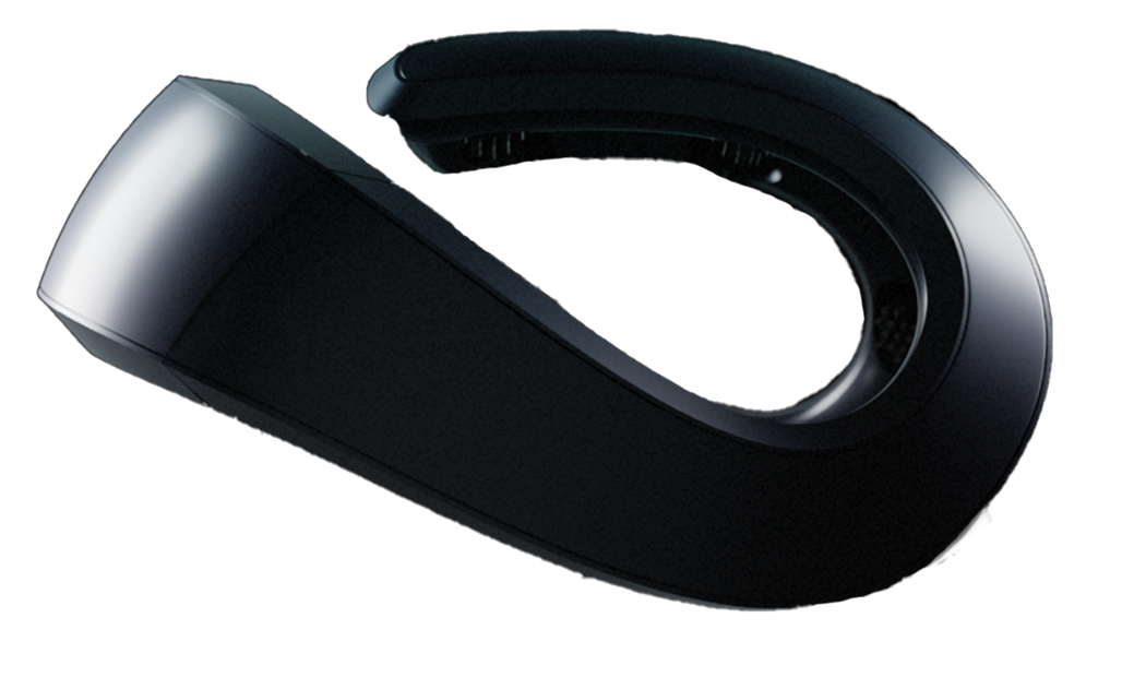
The Neurosity Crown's electrode layout is particularly well-suited for this kind of analysis. The 8 channels span frontal (F5, F6), central (C3, C4), centro-parietal (CP3, CP4), and parieto-occipital (PO3, PO4) cortex across both hemispheres. This gives you the coverage to examine:
- Front-to-back flow: Do frontal regions drive parietal and occipital regions (top-down) or vice versa (bottom-up)?
- Interhemispheric flow: Does the left hemisphere drive the right, or the other way around?
- Regional hubs: Which channel acts as the most influential node in the directed network?
The Crown's 256Hz sampling rate provides sufficient temporal resolution for Granger causality analysis in the frequency bands that matter most for cognition (theta through gamma). And because the Crown exposes raw EEG through its JavaScript and Python SDKs, you can pipe the data directly into analysis tools like MNE-Python, EEGLAB, or custom pipelines using the BrainFlow integration.
On-device processing through the N3 chipset means you can record data without it leaving the device unless you explicitly export it. For researchers analyzing directed connectivity in sensitive contexts, this hardware-level privacy architecture is a genuine advantage over systems that route data through cloud servers.
- Stream raw EEG from the Crown via the Neurosity SDK (JavaScript or Python)
- Segment data into analysis windows (1-4 seconds is typical for stationarity)
- Preprocess each window: bandpass filter, remove artifacts, check stationarity (ADF test)
- Select model order using AIC or BIC
- Fit VAR models and compute pairwise Granger causality (or use spectral decomposition for frequency-resolved analysis)
- Assess significance using surrogate data (phase-shuffling or bootstrap methods)
- Build a directed connectivity matrix and visualize as a network graph
- Repeat across time windows for dynamic connectivity analysis
The Future of Directed Connectivity: Where This Is Heading
The field is moving fast, and several developments are worth watching.
Time-varying Granger causality methods now allow researchers to track how directed connectivity changes on a second-by-second basis. Instead of a static snapshot, you get a movie of information flow evolving in real time as the brain shifts between cognitive states. Combined with consumer EEG devices, this could eventually power applications that detect not just your current brain state but the directed dynamics underlying it.
Machine learning approaches are beginning to complement classical Granger causality. Neural networks can capture nonlinear directed dependencies that VAR models miss, though interpretability remains a challenge. The dream is a method that combines the rigor of Granger causality with the flexibility of deep learning.
Graph-theoretic analysis applied to Granger-causal networks is revealing organizational principles of brain communication. Researchers compute metrics like "causal density," "information transfer hubs," and "directed small-world properties" to characterize how efficiently the brain routes information. Early findings suggest that neurological and psychiatric conditions alter these network properties in specific, detectable ways.
Your Brain Is a Network With a Direction
Here's the thing that Granger causality makes viscerally clear: your brain is not just a collection of active regions. It's a directed communication network. The same set of regions can produce completely different experiences depending on which direction information flows between them.
Top-down frontal-to-sensory flow and you're paying attention, filtering the world through your goals. Bottom-up sensory-to-frontal flow and you're reacting, letting the world capture your focus. The same two endpoints, the same wiring, but the direction of the conversation changes everything.
For most of history, we couldn't see this direction. We could measure brain activity. We could see synchronization. But the flow, the who-speaks-first that determines what you're actually experiencing, was invisible.
Now it isn't. And the tools to see it are no longer locked away in laboratories with six-figure equipment budgets. A well-designed EEG device on your head, a laptop running Python, and the right analysis pipeline can reveal patterns of directed brain communication that were literally unmeasurable 25 years ago.
The question that keeps the field up at night is this: if you could see the direction of information flow in your own brain in real time, what would you do with it? Would you train it? Could you learn to shift from bottom-up reactivity to top-down focus on command? Could a neurofeedback system that shows you not just your brain state but the causal architecture behind it teach you to think differently?
Nobody knows yet. But the tools to find out are here.